I promise to write technical stuff in my blog in a more popular way, just like Olav Laudy. But I have to take my promise. This problem has been bugging me and pushed me to write it for my documentation.
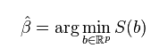
I have been trying to solve some problem using optimization in R, especially the quadratic programming problem. Let’s take a look at the standard formulation of quadratic programming
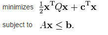
Where x is the optimal parameter that need to be found, Q is the hessian matrix and c is the cost. The second line related to the constraint.
In R, package solve.QP can be used to solve quadratic programming problem. The code to solve the problem is
solve.QP(Dmat, dvec, Amat, bvec, meq=0, factorized=FALSE)
where Dmat is the hessian matrix, dvec is the cost or c, Amat is the A matrix and bvec is the b vector. The meq is used for equality constrain for the top constrain. Factorized is logical flag, if the value is true then the Dmat will pass inverse of R where D=RTR instead of hessian matrix D.
Some example from the CRAN website
##
## Assume we want to minimize: -(0 5 0) %*% b + 1/2 b^T b
## under the constraints: A^T b >= b0
## with b0 = (-8,2,0)^T
## and (-4 2 0)
## A = (-3 1 -2)
## ( 0 0 1)
## we can use solve.QP as follows:
##
Dmat = matrix(0,3,3)
diag(Dmat) = 1
dvec = c(0,5,0)
Amat = matrix(c(-4,-3,0,2,1,0,0,-2,1),3,3)
bvec = c(-8,2,0)
solve.QP(Dmat,dvec,Amat,bvec=bvec)
If we look at it closely, it is apparent that now the inequality constrain signed is now >= instead of <=. This is my first confusion. Why R is change it? Look carefully at the objective function, we can now see that the c vector (dmat) is –(0 5 0). See the minus sign? Yes, that’s the solution. On the first part, x was forced to be negative, while on the second part (quadratic) x is also forced to be negative, but since it is square the negative become positive. That is why the sign of the constrain change to >=, because in the end it is the same thing.
Let see the quadratic programming to solve regression problem. We know that regression optimal parameter are approached using optimization, we want to minimize the error of residual sums of squares (RSS) or S(b) in below equation
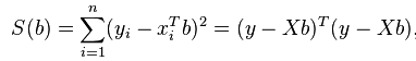
And the parameter beta is

Since this is a convex problem, of first derivative will do the trick. Just for fun, we want to solve it using optimization algorithm. The RSS can be expanded like this
RSS = ( Y - X b )' ( Y - X b )
    = Y Y' - 2 Y' X b + b X' X b
My second confusion dealt with the optimization approach for linear regression problem on this website http://zoonek.free.fr. The code for nonconstrained quadratic optimization in R is as follow
# Sample data
n = 100
x1 = rnorm(n)
x2 = rnorm(n)
y = 1 + x1 + x2 + rnorm(n)
X = cbind( rep(1,n), x1, x2 )

# Regression
r = lm(y ~ x1 + x2)

# Optimization

library(quadprog)
s = solve.QP( t(X) %*% X, t(y) %*% X, matrix(nr=3,nc=0), numeric(), 0 )

coef(r)
s$solution # Identical
see that Dmat is X’ X and coded as t(X) %*% X
and dvec is -2Y’ X and coded as t(y) %*% X
So, where is the value 2 and Y Y’? This is answer, the problem is a separable problem. It means that we can simplify the eqution
min Y Y’ – 2 Y’ X b + b X’ X b is equal to min Y Y’ +2* min(- Y’ X b) + min(b X’ X b).
Since Y Y’ and 2 are constant, it wont affect the optimization thus, the final formulation is
min – Y’ X b + b X’ X b
which is exactly like the code from the website